LabVIEW - Waveform Display Control

We will introduce the use of the first three types of graphic display controls through some examples in the following chapters.

Waveform graphs and waveform charts

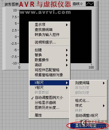
First place a waveform chart on the front panel, then right-click on it, as shown in the figure:

Or right-click and select Properties to see all the options that can be operated on the control, as shown in the figure:

Example 1: Use a waveform chart to display two sets of random numbers.

1. Create a new VI, place a waveform chart on the front panel, and cancel the scale labels of the X-axis and Y-axis, as shown in the figure:

   

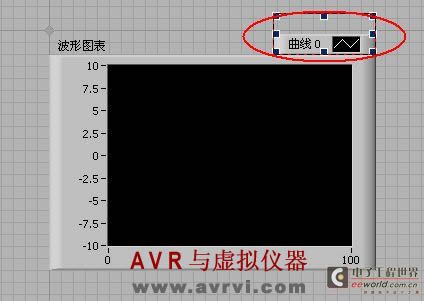
2. Use the positioning tool to drag the border up and down to display two curve legends, as shown in the figure:

   

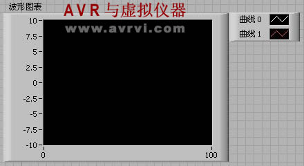
3. Then drag them to the appropriate position. As shown in the figure:

   

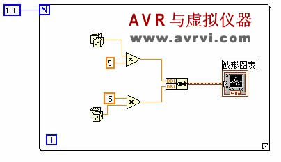
4. Switch to the program flowchart, place a For loop, and set the count terminal value to 100, so that 100 data are generated each time it runs. Place two random number generation functions in the loop body, multiplying by a factor of 5 and -5 respectively. As shown in the figure:

   

The running results are shown in the figure:

Example 2: Temperature critical warning device

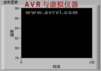
1. Create a new VI, place a waveform chart on the front panel, change the scale label of the Y axis to "Temperature", then choose to hide the legend, and then cancel the automatic adjustment of the Y axis coordinates, as shown in the figure:

2. 

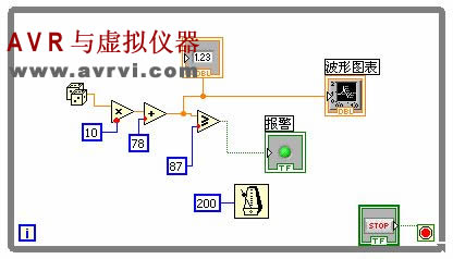
3. Add a Boolean circular indicator light and adjust it to an appropriate size. Change the label content to "Alarm". When the temperature exceeds the critical value, the alarm light will turn on. At the same time, place a stop switch on the front panel.
4. Place the program shown in the figure on the flowchart, add a timing tool, and set the time interval to 200ms. As shown in the figure:

5. 

The running results are shown in the figure:

Waveform

Most of the components and functions of the waveform chart and waveform diagram are similar. The special feature of the waveform chart is that it has a cursor indicator, which can be used to accurately read the data at any point on the waveform curve, making it easier to analyze the characteristic value at a certain moment. As shown in the figure:

Waveform example:

Example 1: The purpose of this example is to use the random number function to generate 100 random data, display them using a waveform graph and a waveform chart, and compare their differences.

1. Create a new VI, place a waveform graph and a waveform chart on the front panel, adjust them to the appropriate size, cancel the legend, cancel the automatic adjustment of the Y scale, set the maximum value to 1, and the minimum value to 0.
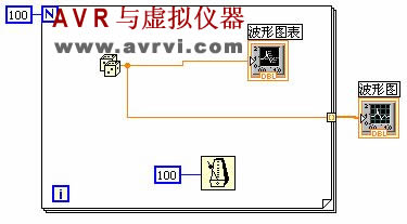
2. Switch to the program flowchart, place a For loop structure, add a random number generation function inside, set the For loop structure count port to 100, and add a timing tool, with each loop interval being 100ms.
3. Connect as shown:

4. 

Run the program, the result is as shown below:

We can clearly see the difference between these two display tools. Their implementation methods and processes are different. It can also be seen in the program flowchart that the waveform chart is generated in the loop body, so that each data point is displayed immediately; while the waveform chart is generated outside the loop body, after 100 data are generated, it jumps out of the loop and then displays the entire data curve at once. When the program runs for the second time, the X-axis scale of the waveform chart will increase from 0 to 99 to 100 to 199, indicating the increase of data points; while the X-axis scale of the waveform chart has not changed, still 0 to 99, indicating that only the current data is displayed. [page]

Example 2: The purpose of this example is to learn how to use the "bundle" package function to set the X-axis scale starting point and interval of the waveform chart.

1. Create a new VI, place a waveform graph on the front panel, and cancel the automatic adjustment of the X-axis so that the generated waveform can fill the entire X-axis scale. Place two numeric input controls at the same time, Xo controls the starting point of the X-axis scale, the data type is I32, and Delta X controls the horizontal interval of the X-axis scale, the data type is DBL.
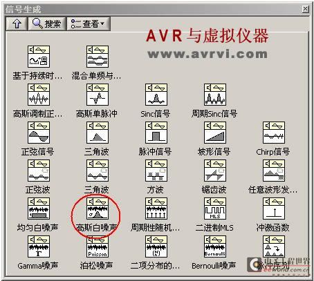
2. Switch to the program flowchart and place a Gaussian white noise function, which is located in Function → Signal Processing → Signal Generation → Gaussian White Noise. As shown in the figure:

3. 

4. Add a "Bundle" function, use the Positioning tool to drag its border into three input ports, and then connect them as shown.

Run, the result is as shown below:

Example 3: The purpose of this example is to learn how to use a cluster array to display data of different lengths and compare it with directly displaying it with a two-dimensional array.

1. Create a new VI, place two waveform graphs on the front panel, change their label contents to "2D Array Display" and "Cluster Array Display" respectively, and set the label font size to 18.
2. Open the program block diagram and add the sine wave function and square wave function, which are located in Function → Signal Processing → Signal Generation → Sine Wave, Square Wave. Assign the sampling ports of these functions 150 and 200 respectively.
3. In the array function, select Create Array Function to combine the outputs of the sine wave and square wave into a two-dimensional array. When introducing arrays, we have learned that when two one-dimensional arrays of different lengths are combined into a two-dimensional array, 0 will be automatically added after the shorter one-dimensional array to make them the same length. Therefore, some meaningless 0s will be added after the sine wave when the graph is displayed.
4. In order to solve the problem of displaying one-dimensional arrays of different lengths, you need to create a cluster array. The method is to use the "Bundle" function to pack the one-dimensional array into a cluster, and then use the Create Array function to create a cluster array. Since each group of data is a cluster, this can solve the problem of displaying one-dimensional arrays of different lengths.

The program flowchart is shown in the figure:

The running results are shown in the figure:

XY Plot

The two waveform displays introduced above: waveform chart and waveform graph can only depict the change curve of a single-valued function with uniformly distributed sample points, because their X-axis only represents the time sequence and is monotonically uniform. To depict the functional relationship between Y and X, you need to use an XY graph. The XY graph is a Cartesian graph in the usual sense. To draw an XY graph, you first need two arrays X and Y, which correspond to the X-axis and Y-axis of the graph respectively, and you need to package the two arrays into a cluster, with the X-axis on the top and the Y-axis on the bottom. The following two examples illustrate the general usage of the XY graph.

The XY graph is located in Controls → New → Graphics → XY Graph, as shown in the figure:

Example 1: Use XY graph to display Lissajous graph.

First, let's briefly introduce the principle of forming Lissajous figures. If we know that the two arrays in the X and Y directions change according to the sinusoidal law (assuming that the number of data points, amplitude and frequency are the same), if their phases are the same, then the Lissajous figure drawn using the XY graph is a 45° oblique line; when the phase difference between them is equal to 90°, it is a circle; in most cases, it is an ellipse.

1. Create a new VI, place an XY graph on the front panel, adjust its border to an appropriate size, and place a numeric input control "Phase Difference".
2. Switch to the block diagram and add two sine wave functions to the block diagram. Connect the "Phase Difference" input control to the "Phase Input" port of the second sine wave function. The default phase is 0.
3. Select the "Bundle" function on the cluster function sub-template to package the two sine signals into a cluster. The first array is used as the data of the X-axis, and the second array is used as the data of the Y-axis. The output of the cluster is connected to the XY graph. As shown in the figure:

Example 2: Using XY graph to draw concentric circles

1. Create a new VI, place an XY graph on the front panel, and make the graph legend display two graph labels.
2. Place a For loop on the program flowchart, assign 360 to the counting terminal, and add sine and cosine functions, which are located in Functions → Mathematics → Basic and Special Functions → Trigonometric Functions → Sine, Cosine.
3. Select "Bundle" to package the function, and cluster the pair of sine and cosine values ​​generated in each loop into a cluster. After the loop ends, these 360 ​​clusters are combined into a cluster function.
4. Because the display mechanism of the XY graph determines that its input must be a cluster, we need to use the "Bundle" packaging function again to convert the two cluster arrays into clusters, and finally use the "Create Array" function to form a cluster array. The program flowchart is as follows:

The running results are shown in the figure:

Labview also provides us with another XY diagram, which is the Express XY diagram. When we switch to the program flowchart, we will see that it is easier to use than the simple XY diagram on the program flowchart. From the diagram we can also see that it has two input ports, and the input can be either a single value or an array. We will not introduce it in detail here.